From “Method Development, Optimization and Trouble Shooting for High Performance Capillary Electrophoresis”
Theoretical Plates: Efficiency
By what methods can one keep score in Separation Science? Efficiency! If our method achieves several hundred thousand theoretical plates, we are doing well and have a good separation. If our method achieves only a few theoretical plates we must change the method or the separation technique.
Understanding Theoretical Plate Counts
The theoretical, maximum plate count for any separation can be calculated from Professor James Jorgenson’s equation where:
| N | = the number of theoretical plates |
| µep | = electrophoretic mobility |
| E | = field strength |
| Ld | = length of the capillary to detector |
| Dm | = solute diffusion coefficient |
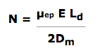
Time related diffusion is the only source of band broadening (peak variance) allowed by this equation. Although this equation predicts approximately 1,000,000 theoretical plates as the theoretical maximum, when we add other sources of band broadening, then N naturally declines. HPCE has inherently high theoretical plates.
A natural dilemma in HPCE
A dilemma in HPCE is how to maintain its inherent efficiency and the more efficient a method or process, the more difficult that becomes. This is due to the additivity of variances, which can be stated as:
O2 tot = O2diff + o2inj + o2det + o2all others +…
| O2tot | = total source of band broadening |
| O2diff | = diffusion coefficient |
| O2inj | = band broadening due to injection limitations |
| O2det | = band broadening due to detection limitations |
| O2all others | = all other sources of band broadening |
When the diffusion coefficient is very low, we are challenged to maintain very low variances for all other potential sources of band broadening. Thus the adventure begins for the adventurous scientist or student.
Other sources of band broadening
Each of the following sources of band broadening are discussed and solutions and tips are offered to optimize each source.
Click on the Links below for the explanation.
- Detection
- Detector Time Constant
- Injection
- Wall Effects
- Joule Heating
- Electrodispersion
- Sample's Ionic Strength
- Broken Column/Capillary Ends
- BGE Containers Not Level
Simple Solutions to Natural Sources of Band Broadening in HPCE
Injection and Detection Sources of Band Broadening
Detection Volume
In HPCE (unlike in HPLC), the path length of the detector is defined by the capillary diameter. Therefore the illuminated volume of the detector region is very small (<1nL) and is not usually controllable by the user. Unless one uses an extended path length flow cell there is very little one can do about controlling band broadening sources from the detector. If you are using an extended path or a “bubble cell” and are experiencing band broadening, you can use a standard diameter capillary to reduce the band broadening that may occur. Also, there is very little contribution to band broadening from the detector with exception to Detector time constants.
Back to List of Links
Detector Time Constants
Relatively short detection time constants are required in HPCE due to the very sharp peaks that normally occur. Set your detector time constants to a value that is 10-20% of the peak width. Longer time constants will result in band broadening, tailing and loss of resolution. The exact peak shape obtained in an over-filtered state is dependant on the type of filtering used in the detector.
The figure below is an example of how Detector Time Constants can affect efficiency and signal to noise ratios.
Note the decline in peak height for the peaks when the rise time is beyond 0.2s. For the 2s rise time, the peak shows unacceptable tailing. The optimal setting is 1s in this figure. If the selected time is too short, then we observe an unnecessary decline in signal to noise ratio.
Back to List of Links
Injection Volume
Injection size is a far more important contribution to band broadening. The following derivative of the Jorgenson Theoretical Plate equation defines variance (band broadening) due to injection volumes.
| N | = number of theoretical plates |
| Ld | = length of the capillary to the detector |
| O2tot | = total source of band broadening |
N = (Ld/Otot)2
| where O2tot | = 2Dm t + w2/12 |
| w | = width of injection zone |
In the following chart, we show the decline in efficiency as injection size is increased for a large and small molecule using a 50cm capillary with a solute migration of 10 min. When filling the capillary with 2% of its volume with sample, about 1% of the theoretical maximum plate count is found for a large molecule. For a small molecule, we reach 10% of the theoretical maximum. Thus, even very small injections can result in substantial losses in efficiency. This argument presumes that we are injecting with the sample dissolved in the BGE. Make as small of an injection as possible.
Impact of the injection zone length on the number of Theoretical Plates.
Capillary Length: 50cm
Migration time 10 min.
Diffusion Coefficient: 10-5/cm2/s (Lower curve) & 10-6/cm2/s (Upper curve)
Wall Interactions
In HPCE, solutes can adhere to the capillary wall through electrostatic and hydrophobic interactions. It is fundamental to the high efficiency of HPCE that the process operates with zero retention. As an note of interest, in HPLC, the restricted mass transport between liquid and solid phase is the most important limiting factor to higher efficiency.
“The Random Walk Method”
More sophisticated models have appeared in the literature than “The Random Walk Method” which is a theory that considers a solute moving down the capillary in discrete steps. This is a good first approximation.
| ta | = time for adsorption |
| td | = time for desorption |
Band Broadening (Peak Variance) is:
| O2s = 2 { k' }2 | |
| VeptaL | |
| 1+k' | |
Retention occurs whenever td > ta. Tailing occurs since a desorbed solute does not return at once to the buffer or bulk flow solution. Retained solutes have a migration velocity of zero. Solutes in the buffer or bulk flow solution move at a rate determined by their migration velocity and thus move ahead of retained solutes.
Evaluation of this function for a 1,000,000 theoretical plate separation illustrates that to achieve maximum efficiency for HPCE (CZE), k’ must be near zero.
Even modest retention can lead to severe band broadening. Appropriate buffer additives, column coatings or dynamic coatings may be required to minimize this form of band broadening.
It is suggested that during method development, you first undertake reducing or eliminating wall effects before undertaking other optimization studies. These effects are not subtle. Often when one ignores this suggestion, there is much time and effort wasted.
Wall effects can lead to tailed peaks, broadened peaks or in severe cases, no peaks at all. One sign that wall effects are occurring is the when you have one sharp peak, one broad peak and another sharp peak. This may indicate that you have multiple overlapping solutes. It is also possible that your solutes may be experiencing selective adsorption.
Back to List of Links
Joule Heating
The production of heat in the capillary due to frictional forces of colliding ions and solute molecules is called Joule Heating. When Joule heating occurs, a parabolic temperature gradient is formed within the capillary. Due to the temperature gradient, a viscosity gradient is formed as well.
Mobility is inversely proportional to the viscosity of the BGE (back ground electrolyte), ions in the center of the capillary will migrate faster than those closer to the wall. If Joule heating is uncontrolled, the band broadening can be very substantial.
A simple tool is offered to reduce the significance of Joule Heating: an Ohm’s Law Plot.
An Ohm’s Law Plot is simply a graph of voltage to current. The point at which there is a positive deviation (about 5%) from linearity, is the optimal voltage for the separation.
Whenever you adjust experimental conditions in your method, you should run an Ohm’s Law Plot since the optimal voltage (minimal Joule Heating) is dependant upon capillary diameter, capillary length, BGE concentration, BGE ionic mobilities, temperature of the system and efficiency of the instrument’s cooling system.
Ohm’s Law Plot for an air cooled (A) and liquid Cooled (B) systems at 10C. From this graph, you can see the merits of a liquid cooled system versus an air cooled system. Higher voltages can be used before linearity begins to deteriorate.
Electrodispersion
When the solute concentration reaches the BGE concentration, a form of band broadening known as “Electrodispersion” frequently occurs. This break down of efficiency can be seen in the “saw tooth” shaped peaks when using indirect detection, performing micro preparative separations and at the higher solute concentrations of a calibration curve.
Electrodispersion occurs when there is a difference in the conductivity of a solute band compared to that of the BGE. From Ohm’s law for a series circuit, we can write:
E = IR1 + IR2 + IR3…+ IRn
Thus a highly conductive solute band (will have high mobility) generates a low resistance and a low voltage drop compared to the field over the BGE. The reverse is true for a solute band with low conductivity (low mobility).
This is an example of the electropherograms that you will see when Electrodispersion is occurring.
µsolute > mBGE
Csolute approaches CBGE
At the front of the zone, diffused solute ions become exposed to the higher electric field strength over the BGE and thus accelerate away from the slowly migrating solute ions that comprise the balance of the solute ions. This leads to band broadening at the front of the zone.
At the rear of the zone, solute ions are exposed to higher electric field strength across from the BGE but in this case, they recombine with the slowly migrating ions since their mobility is directed towards the cathode.
For low mobility solutes, the opposite it true. The band broadening occurs at the rear of the sample zone.
In the case where the mobility of the solute equals the mobility of the BGE does no band broadening occur.
To achieve high efficiency and reduce effects due to Electrodispersion, use the following suggestions:
-
Dilute the Sample
This works well when sensitivity is not a problem. -
Increase the concentration of BGE (i.e. 25mM to 50mM)
This works well only to the point where Joule heating becomes an issue. -
Reduce the diameter of the capillary.
This works well when sensitivity is not a problem. -
Match the mobility of the BGE co-ion to the solute mobility
This is very important when performing indirect detection since it is not possible to increase the concentration beyond a few milli-molar. Sometimes this is difficult since not all compounds are listed in available tables of matching mobilities.
Electrodispersion is normally easy to cope with. When developing a method, be sure that you have good, solid resolution so that you can deal with any band broadening that may occur since quantification is not affected as long as the integration parameters are properly set and the resolution is adequate.
When performing trace analysis CE, it may be necessary to “mobility match” your BGE co-ion to the major component in the separation.
Electrodispersion increase the linear dynamic range for quantitation. To totally eliminate Electrodispersion, the solute concentration must be a factor of fifty (lower) than the BGE and substantial band broadening does not occur until the solute concentration is much higher.
Back to List of Links
Sample's Ionic Strength
For many samples, all that is required is to “dilute and shoot”. When complex matrices or trace analysis is required, good sample preparation pays dividends in many ways.
Desalting of samples is important to enable stacking to occur. In some cases, the salt concentration may be so high that band broadening due to “anti-stacking” is significant. While the ultimate goal is to have on-line desalting, there are no devices or technology on the market to accomplish this as of yet.
Spin down Biomolecules such as proteins in an ultracentrifuge and make a “pellet”. Discard the supernatant and re-suspend the protein in BGE or a diluted version of the BGE/run buffer. Of course, further cleanup is possible with SPE or an affinity column of some type.
Back to List
Broken Column/Capillary Ends
If the injection side of the capillary or the column is not cut squarely, you may see peak tailing for high efficiency separations. If a well behaved separation suddenly exhibits tailing, examine the end of the column/capillary under magnification. Occasionally, the column/capillary end snaps if it hits a sample or BGE vial closure off-center. If it is not square, re-cut or replace the column/capillary. The amount of band broadening observed is more than can be expected from other volumetric factors alone.
Back to List of Links
Siphoning due to BGE Levels that are not level
Siphoning is a form of hydrodynamic band broadening which only occurs when the fluid levels in the inlet and the outlet reservoirs differ significantly. It is easily remedied once you recognize this. Siphoning is usually problematic when using 75m column/capillaries or larger. This is due to the fact that the flow-rate of the liquid in a capillary tube is directly proportional to the forth power of the capillary diameter.
Back to List of Links